


Detecting Silent Model Decay: A Production Guide to Quantifying Data & Concept Drift
In real-world data science, models rarely fail loudly with crash stack traces. They degrade silently because the statistical distribution of the incoming production features or the underlying relationship between inputs and targets shifts over time.
Relying on quarterly manual re-evaluations is too slow, and waiting for ground-truth labels can take weeks or months. Production data engineering requires an automated, statistical telemetry pipeline to catch drift in flight.
Here is a practical, step-by-step tutorial on implementing statistical drift detection for live inference pipelines.1. Separate Covariate Shift from Concept Shift Before choosing metrics, isolate the exact failure mode you are monitoring:
Covariate (Feature) Shift: The distribution of inputs changes ($P(X)$ changes), but the conditional relationship $P(Y \mid X)$ remains intact (e.g., user demographics skew younger, but purchasing behavior per age group remains stable).Concept Shift: The relationship between features and labels changes ($P(Y \mid X)$ changes), even if input distributions look identical (e.g., macroeconomic inflation changes what constitutes a "high-risk" loan amount).Prior Probability Shift: The target distribution changes ($P(Y)$ changes), common during seasonal demand spikes.2. Implement Statistical Distance Tests per Feature Type Never use simple mean and variance checks—they easily mask multimodal distributions and variance spikes. Segment your feature store into two testing tracks:
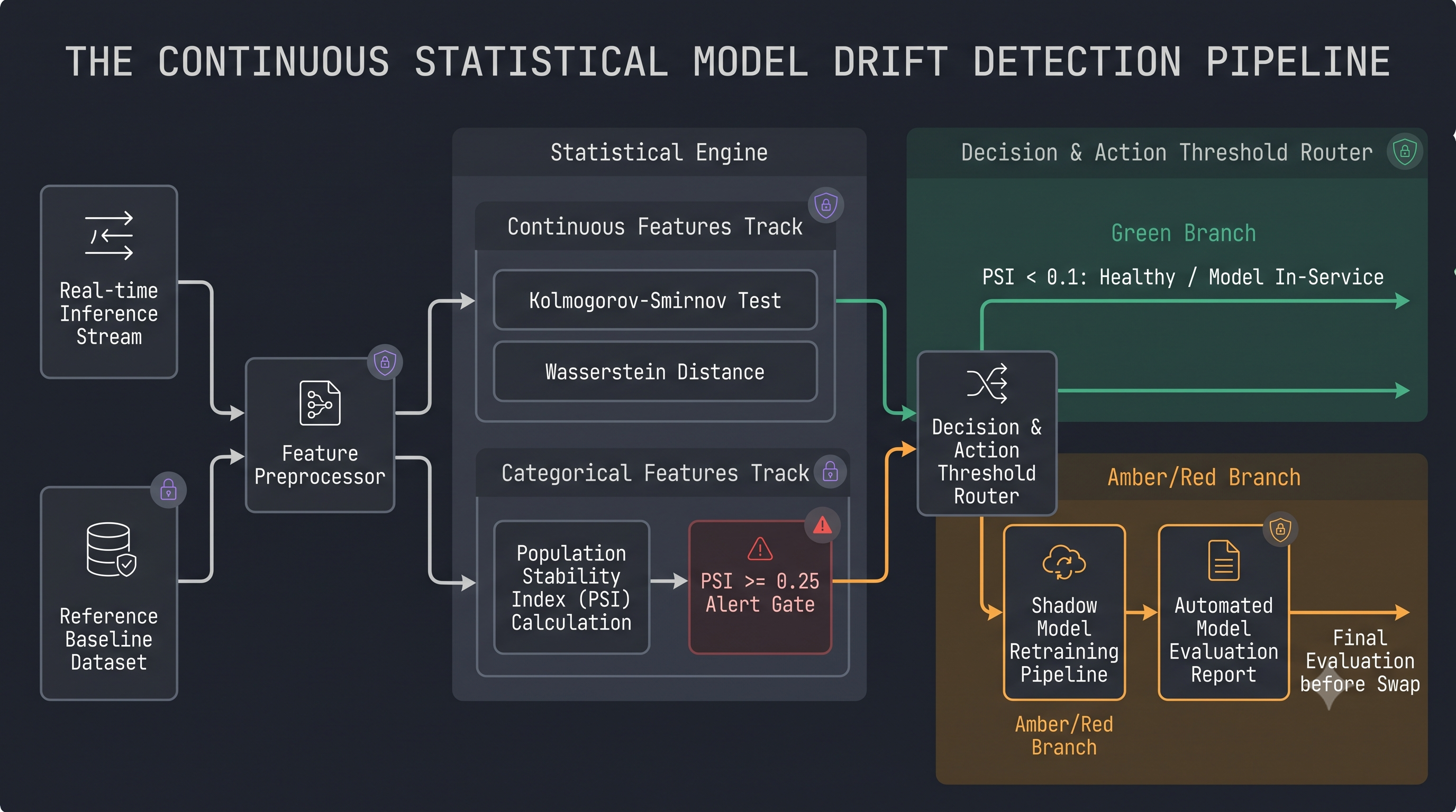
Continuous Features (Kolmogorov-Smirnov & Wasserstein Distance):Use the two-sample Kolmogorov-Smirnov (KS) test to compare the cumulative distribution function (CDF) of production samples against your training baseline.
Supplement with Wasserstein (Earth Mover's) Distance for an absolute, unit-interpretable metric indicating the work needed to transform the production distribution into the baseline.
Categorical Features (Population Stability Index - PSI):Group features into reference buckets and calculate PSI:$$\text{PSI} = \sum \left( \% \text{ Actual} - \% \text{ Expected} \right) \times \ln\left( \frac{\% \text{ Actual}}{\% \text{ Expected}} \right)$$Evaluation Rules:$\text{PSI} < 0.1$: Distribution stable; no action needed.$0.1 \le \text{PSI} < 0.25$: Moderate drift; flag for inspection.$\text{PSI} \ge 0.25$: Significant shift; trigger alert and review pipeline.3. Mitigate Sample Size Sensitivity with Windowed Baselines Statistical tests (like KS and Chi-square) are notoriously sensitive to huge sample sizes: with 500,000 requests, even a trivial, harmless fluctuation yields $p < 0.001$.Use sliding time windows (e.g., rolling 7-day batches) compared against a curated reference window (the model’s gold validation set) rather than an expanding historic pool.
Rely on effect-size metrics (such as PSI or normalized Wasserstein distance) as your primary alert triggers, using $p$-values strictly as secondary filters.4. Wire Drift Thresholds to Automated Retraining Triggers Drift detection is only valuable if it drives operational action:
When multiple critical features breach $\text{PSI} \ge 0.25$, trigger an automated pipeline (via Airflow, Prefect, or Kubeflow) to pull fresh labeled ground truth from recent partitions.
Automatically retrain a shadow candidate model, evaluate performance against current production data, and publish a comparative evaluation report before human sign-off on promotion.
Key Takeaways
Differentiate Shifts: Identify whether you are fighting feature distribution drift ($P(X)$) or fundamental concept decay ($P(Y \mid X)$).Pick the Right Test: Use KS/Wasserstein for continuous features and Population Stability Index (PSI) for categorical inputs.
Effect Size Over $p$-values: Avoid false alarms caused by sample size inflation by alerting on effect sizes ($\text{PSI} > 0.2\() rather than raw\)p$-values.
Automate the Feedback Loop: Connect statistical alerts directly to shadow retraining and validation pipelines.
CTA
How do you track silent model degradation in your production pipelines?Do you rely on dedicated open-source drift frameworks (like Evidently AI, Great Expectations, or NannyML), custom statistical scripts, or downstream business KPIs? Share your monitoring setup, threshold heuristics, and failure stories below.
In real-world data science, models rarely fail loudly with crash stack traces. They degrade silently because the statistical distribution of the incoming production features or the underlying relationship between inputs and targets shifts over time.
Relying on quarterly manual re-evaluations is too slow, and waiting for ground-truth labels can take weeks or months. Production data engineering requires an automated, statistical telemetry pipeline to catch drift in flight.
Here is a practical, step-by-step tutorial on implementing statistical drift detection for live inference pipelines.1. Separate Covariate Shift from Concept Shift Before choosing metrics, isolate the exact failure mode you are monitoring:
Covariate (Feature) Shift: The distribution of inputs changes ($P(X)$ changes), but the conditional relationship $P(Y \mid X)$ remains intact (e.g., user demographics skew younger, but purchasing behavior per age group remains stable).Concept Shift: The relationship between features and labels changes ($P(Y \mid X)$ changes), even if input distributions look identical (e.g., macroeconomic inflation changes what constitutes a "high-risk" loan amount).Prior Probability Shift: The target distribution changes ($P(Y)$ changes), common during seasonal demand spikes.2. Implement Statistical Distance Tests per Feature Type Never use simple mean and variance checks—they easily mask multimodal distributions and variance spikes. Segment your feature store into two testing tracks:
Continuous Features (Kolmogorov-Smirnov & Wasserstein Distance):Use the two-sample Kolmogorov-Smirnov (KS) test to compare the cumulative distribution function (CDF) of production samples against your training baseline.
Supplement with Wasserstein (Earth Mover's) Distance for an absolute, unit-interpretable metric indicating the work needed to transform the production distribution into the baseline.
Categorical Features (Population Stability Index - PSI):Group features into reference buckets and calculate PSI:$$\text{PSI} = \sum \left( \% \text{ Actual} - \% \text{ Expected} \right) \times \ln\left( \frac{\% \text{ Actual}}{\% \text{ Expected}} \right)$$Evaluation Rules:$\text{PSI} < 0.1$: Distribution stable; no action needed.$0.1 \le \text{PSI} < 0.25$: Moderate drift; flag for inspection.$\text{PSI} \ge 0.25$: Significant shift; trigger alert and review pipeline.3. Mitigate Sample Size Sensitivity with Windowed Baselines Statistical tests (like KS and Chi-square) are notoriously sensitive to huge sample sizes: with 500,000 requests, even a trivial, harmless fluctuation yields $p < 0.001$.Use sliding time windows (e.g., rolling 7-day batches) compared against a curated reference window (the model’s gold validation set) rather than an expanding historic pool.
Rely on effect-size metrics (such as PSI or normalized Wasserstein distance) as your primary alert triggers, using $p$-values strictly as secondary filters.4. Wire Drift Thresholds to Automated Retraining Triggers Drift detection is only valuable if it drives operational action:
When multiple critical features breach $\text{PSI} \ge 0.25$, trigger an automated pipeline (via Airflow, Prefect, or Kubeflow) to pull fresh labeled ground truth from recent partitions.
Automatically retrain a shadow candidate model, evaluate performance against current production data, and publish a comparative evaluation report before human sign-off on promotion.
Key Takeaways
Differentiate Shifts: Identify whether you are fighting feature distribution drift ($P(X)$) or fundamental concept decay ($P(Y \mid X)$).Pick the Right Test: Use KS/Wasserstein for continuous features and Population Stability Index (PSI) for categorical inputs.
Effect Size Over $p$-values: Avoid false alarms caused by sample size inflation by alerting on effect sizes ($\text{PSI} > 0.2\() rather than raw\)p$-values.
Automate the Feedback Loop: Connect statistical alerts directly to shadow retraining and validation pipelines.
CTA
How do you track silent model degradation in your production pipelines?Do you rely on dedicated open-source drift frameworks (like Evidently AI, Great Expectations, or NannyML), custom statistical scripts, or downstream business KPIs? Share your monitoring setup, threshold heuristics, and failure stories below.
Detecting Silent Model Decay: A Production Guide to Quantifying Data & Concept Drift
In real-world data science, models rarely fail loudly with crash stack traces. They degrade silently because the statistical distribution of the incoming production features or the underlying relationship between inputs and targets shifts over time.
Relying on quarterly manual re-evaluations is too slow, and waiting for ground-truth labels can take weeks or months. Production data engineering requires an automated, statistical telemetry pipeline to catch drift in flight.
Here is a practical, step-by-step tutorial on implementing statistical drift detection for live inference pipelines.1. Separate Covariate Shift from Concept Shift Before choosing metrics, isolate the exact failure mode you are monitoring:
Covariate (Feature) Shift: The distribution of inputs changes ($P(X)$ changes), but the conditional relationship $P(Y \mid X)$ remains intact (e.g., user demographics skew younger, but purchasing behavior per age group remains stable).Concept Shift: The relationship between features and labels changes ($P(Y \mid X)$ changes), even if input distributions look identical (e.g., macroeconomic inflation changes what constitutes a "high-risk" loan amount).Prior Probability Shift: The target distribution changes ($P(Y)$ changes), common during seasonal demand spikes.2. Implement Statistical Distance Tests per Feature Type Never use simple mean and variance checks—they easily mask multimodal distributions and variance spikes. Segment your feature store into two testing tracks:
Continuous Features (Kolmogorov-Smirnov & Wasserstein Distance):Use the two-sample Kolmogorov-Smirnov (KS) test to compare the cumulative distribution function (CDF) of production samples against your training baseline.
Supplement with Wasserstein (Earth Mover's) Distance for an absolute, unit-interpretable metric indicating the work needed to transform the production distribution into the baseline.
Categorical Features (Population Stability Index - PSI):Group features into reference buckets and calculate PSI:$$\text{PSI} = \sum \left( \% \text{ Actual} - \% \text{ Expected} \right) \times \ln\left( \frac{\% \text{ Actual}}{\% \text{ Expected}} \right)$$Evaluation Rules:$\text{PSI} < 0.1$: Distribution stable; no action needed.$0.1 \le \text{PSI} < 0.25$: Moderate drift; flag for inspection.$\text{PSI} \ge 0.25$: Significant shift; trigger alert and review pipeline.3. Mitigate Sample Size Sensitivity with Windowed Baselines Statistical tests (like KS and Chi-square) are notoriously sensitive to huge sample sizes: with 500,000 requests, even a trivial, harmless fluctuation yields $p < 0.001$.Use sliding time windows (e.g., rolling 7-day batches) compared against a curated reference window (the model’s gold validation set) rather than an expanding historic pool.
Rely on effect-size metrics (such as PSI or normalized Wasserstein distance) as your primary alert triggers, using $p$-values strictly as secondary filters.4. Wire Drift Thresholds to Automated Retraining Triggers Drift detection is only valuable if it drives operational action:
When multiple critical features breach $\text{PSI} \ge 0.25$, trigger an automated pipeline (via Airflow, Prefect, or Kubeflow) to pull fresh labeled ground truth from recent partitions.
Automatically retrain a shadow candidate model, evaluate performance against current production data, and publish a comparative evaluation report before human sign-off on promotion.
Key Takeaways
Differentiate Shifts: Identify whether you are fighting feature distribution drift ($P(X)$) or fundamental concept decay ($P(Y \mid X)$).Pick the Right Test: Use KS/Wasserstein for continuous features and Population Stability Index (PSI) for categorical inputs.
Effect Size Over $p$-values: Avoid false alarms caused by sample size inflation by alerting on effect sizes ($\text{PSI} > 0.2\() rather than raw\)p$-values.
Automate the Feedback Loop: Connect statistical alerts directly to shadow retraining and validation pipelines.
CTA
How do you track silent model degradation in your production pipelines?Do you rely on dedicated open-source drift frameworks (like Evidently AI, Great Expectations, or NannyML), custom statistical scripts, or downstream business KPIs? Share your monitoring setup, threshold heuristics, and failure stories below.

 Arabic
 French
 Spanish
 Portuguese
 Deutsch
 Turkish
 Dutch
Dutch
 Italiano
 Russian
 Romaian
 Portuguese (Brazil)
 Greek
Greek