


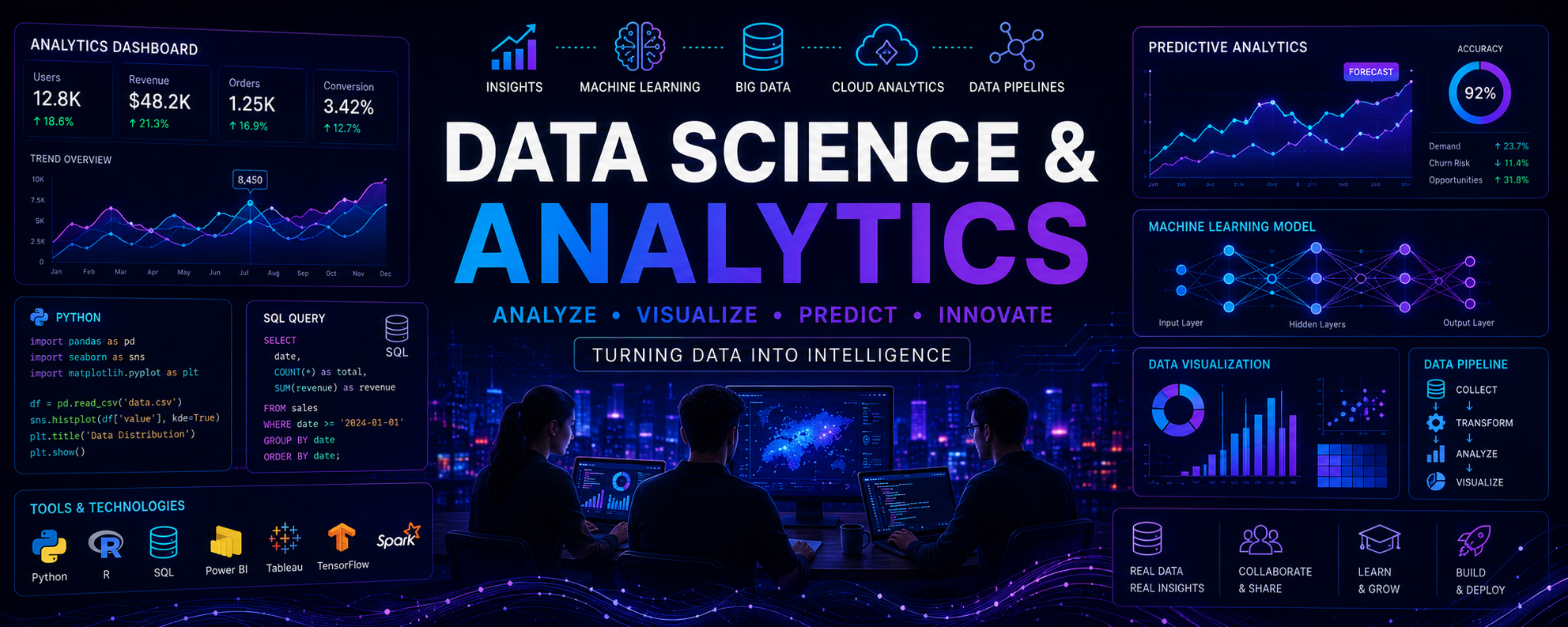

Data Science & Analytics is a Techawks community for students, professionals, researchers, and enthusiasts who want to explore the world of data, artificial intelligence, machine learning, and business analytics. Learn how to collect, analyze, visualize, and transform data into meaningful insights.
Discover practical tutorials, datasets, analytics tools, Python and SQL techniques, machine learning projects, dashboards, career guidance, certifications, and industry trends. Connect with others to share knowledge, solve real-world problems, and build data-driven skills for the future.
Discover practical tutorials, datasets, analytics tools, Python and SQL techniques, machine learning projects, dashboards, career guidance, certifications, and industry trends. Connect with others to share knowledge, solve real-world problems, and build data-driven skills for the future.
-
Groupe public
-
64 Articles
-
64 Photos
-
0 Vidéos
-
Aperçu
-
Science and Technology
Rechercher

 English
 Arabic
 Spanish
 Portuguese
 Deutsch
 Turkish
 Dutch
Dutch
 Italiano
 Russian
 Romaian
 Portuguese (Brazil)
 Greek
Greek
Mises à jour récentes
-
Resizing Stateful Streaming Without Checkpoint Wipeouts: The End of Cold Replays
Scaling stateless stream processing (mapping, filtering, schema casting) is trivial—you spin up more consumer nodes. Scaling stateful operations (sessionization, rolling aggregations, continuous watermarking, and real-time anomaly detection) has historically been an architectural headache.
When state is tied directly to physical partition geometry via serialized checkpoint directories (such as RocksDB state stores), altering parallel task slots typically breaks partition-to-state affinity. If your stream lags during an unexpected surge, your options used to be brutal: over-provision 24/7 or endure downtime while rehydrating multi-gigabyte state buffers.
Recent engine upgrades across the streaming ecosystem—most notably dynamic partition reassignment and checkpoint-preserving rescaling in modern Spark Structured Streaming and Flink deployments—fundamentally change how data teams manage live ML inference and real-time aggregations.
Key Technical Takeaway: Decoupled Key-Group Routing
Instead of binding checkpointed state directly to partition IDs:
Virtual Key-Grouping: Continuous aggregations distribute incoming keys across a fixed, oversized virtual key-space (e.g., 1024 virtual buckets) rather than hardcoded physical worker partitions.
State Store Decoupling: When worker capacity scales from 4 to 16 executors, the streaming runtime re-assigns virtual key ranges across the newly allocated workers.
Differential State Rehydration: Workers fetch only their designated slice of the checkpoint state asynchronously from object storage, avoiding total pipeline stops and eliminating manual consumer group offset resets.
Operational Checklist: Evaluating Stateful Resiliency
Check State Serialization Overhead: Ensure your stateful operators use native memory formats or off-heap engines to prevent JVM garbage-collection pauses during rebalance.
Audit Watermark Lateness Policies: Tighten allowed lateness windows. Storing unnecessary out-of-order records inflates checkpoint size, making live worker re-allocation drag.
Implement Asynchronous Snapshotting: Decouple state persistence from message commit loops so scaling operations don't cascade backpressure into Kafka or event-bus ingest layers.
Discussion Question
How does your team handle partition scaling for stateful streaming pipelines during volume spikes—do you over-provision baseline compute, rely on dynamic slot reassignment, or run scheduled checkpoint rebuilds?
CTA
Share your streaming architecture tradeoffs and war stories in the comments. Let's dig into how your team balances state durability, low latency, and cloud infrastructure costs.Resizing Stateful Streaming Without Checkpoint Wipeouts: The End of Cold Replays Scaling stateless stream processing (mapping, filtering, schema casting) is trivial—you spin up more consumer nodes. Scaling stateful operations (sessionization, rolling aggregations, continuous watermarking, and real-time anomaly detection) has historically been an architectural headache. When state is tied directly to physical partition geometry via serialized checkpoint directories (such as RocksDB state stores), altering parallel task slots typically breaks partition-to-state affinity. If your stream lags during an unexpected surge, your options used to be brutal: over-provision 24/7 or endure downtime while rehydrating multi-gigabyte state buffers. Recent engine upgrades across the streaming ecosystem—most notably dynamic partition reassignment and checkpoint-preserving rescaling in modern Spark Structured Streaming and Flink deployments—fundamentally change how data teams manage live ML inference and real-time aggregations. Key Technical Takeaway: Decoupled Key-Group Routing Instead of binding checkpointed state directly to partition IDs: Virtual Key-Grouping: Continuous aggregations distribute incoming keys across a fixed, oversized virtual key-space (e.g., 1024 virtual buckets) rather than hardcoded physical worker partitions. State Store Decoupling: When worker capacity scales from 4 to 16 executors, the streaming runtime re-assigns virtual key ranges across the newly allocated workers. Differential State Rehydration: Workers fetch only their designated slice of the checkpoint state asynchronously from object storage, avoiding total pipeline stops and eliminating manual consumer group offset resets. Operational Checklist: Evaluating Stateful Resiliency Check State Serialization Overhead: Ensure your stateful operators use native memory formats or off-heap engines to prevent JVM garbage-collection pauses during rebalance. Audit Watermark Lateness Policies: Tighten allowed lateness windows. Storing unnecessary out-of-order records inflates checkpoint size, making live worker re-allocation drag. Implement Asynchronous Snapshotting: Decouple state persistence from message commit loops so scaling operations don't cascade backpressure into Kafka or event-bus ingest layers. Discussion Question How does your team handle partition scaling for stateful streaming pipelines during volume spikes—do you over-provision baseline compute, rely on dynamic slot reassignment, or run scheduled checkpoint rebuilds? CTA Share your streaming architecture tradeoffs and war stories in the comments. Let's dig into how your team balances state durability, low latency, and cloud infrastructure costs.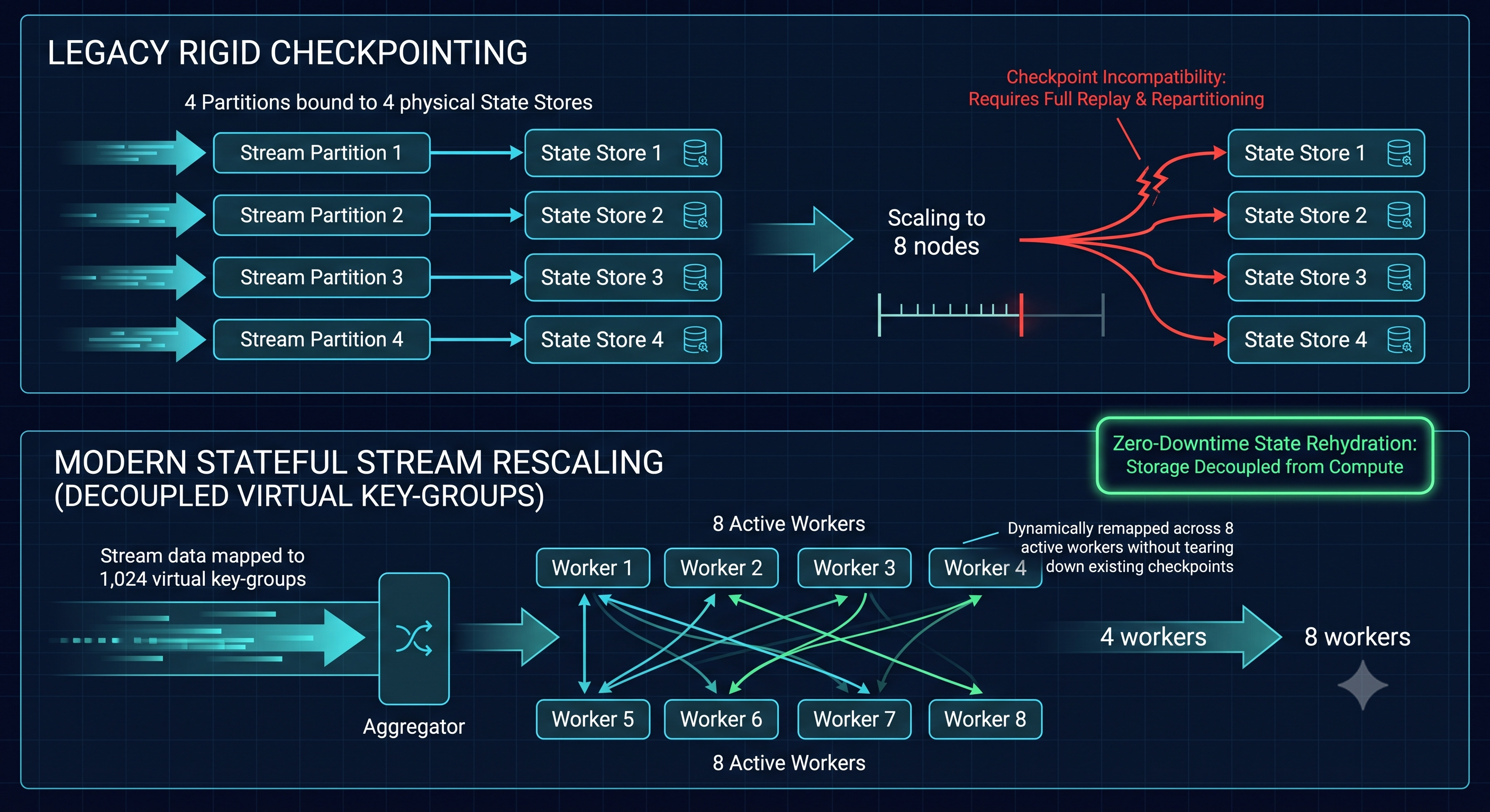 0 Commentaires 0 Parts 11 Vue 0 Aperçu
 -
Feature Store vs. Database View: Where Should Your Real-Time Feature Logic Actually Live?
When scaling production machine learning, the boundary between data engineering and machine learning operations often blurs around one critical component: feature transformation and retrieval.
A common debate among data platforms is whether to invest in a dedicated Feature Store (like Feast, Hopsworks, or managed cloud alternatives) or rely on Optimized Database Views/dbt pipelines running against an analytical warehouse or low-latency operational store (like Redis, DynamoDB, or PostgreSQL).
Here is how the trade-offs break down in practice:
Point-in-Time Correctness (Time-Travel Joins)
Database Views: Complex to write and computationally expensive when reconstructing feature values as of an exact timestamp without data leakage.
Feature Stores: Built natively with point-in-time correctness, joining historical labels with the exact feature values that were valid at prediction time.
Training-Serving Skew
Database Views: Often require dual implementations: SQL for historical training batches, and Python/Go microservices for low-latency production inference. Any subtle divergence between these definitions causes silent model degradation.
Feature Stores: Provide a single definition interface. Features are computed once and pushed to both the offline store (for model training) and the low-latency online store (for real-time inference).
Latency and Query Semantics
Database Views: Complex aggregations (e.g., number of transactions in the last 10 minutes) can struggle to maintain sub-50ms p99 SLA under high-concurrency production load unless heavily pre-indexed or cached.
Feature Stores: Pre-materialize real-time entity features directly into an in-memory key-value cache, reducing inference lookup to single-digit milliseconds.
The catch? A feature store introduces platform complexity, extra synchronization layers, and maintenance overhead that smaller teams may not need if their inference workflows are purely batch-driven.
Key Takeaways
Stick to DB Views/dbt if your inference is batch-only, features update on daily/hourly schedules, and latency under 100ms is not a hard constraint.
Adopt a Feature Store when you have online/real-time inference, multiple models sharing the same entity features, or recurring issues with data leakage during training set creation.
Consistency across the offline/online boundary is usually the deciding factor, not just storage speed.
CTA
Where does your team draw the line?
If you are currently serving models in production: Have you migrated to a dedicated feature store, or are you successfully managing offline-to-online parity using warehouse transformations and key-value tables? Let's break down the architectural choices in the comments.Feature Store vs. Database View: Where Should Your Real-Time Feature Logic Actually Live? When scaling production machine learning, the boundary between data engineering and machine learning operations often blurs around one critical component: feature transformation and retrieval. A common debate among data platforms is whether to invest in a dedicated Feature Store (like Feast, Hopsworks, or managed cloud alternatives) or rely on Optimized Database Views/dbt pipelines running against an analytical warehouse or low-latency operational store (like Redis, DynamoDB, or PostgreSQL). Here is how the trade-offs break down in practice: Point-in-Time Correctness (Time-Travel Joins) Database Views: Complex to write and computationally expensive when reconstructing feature values as of an exact timestamp without data leakage. Feature Stores: Built natively with point-in-time correctness, joining historical labels with the exact feature values that were valid at prediction time. Training-Serving Skew Database Views: Often require dual implementations: SQL for historical training batches, and Python/Go microservices for low-latency production inference. Any subtle divergence between these definitions causes silent model degradation. Feature Stores: Provide a single definition interface. Features are computed once and pushed to both the offline store (for model training) and the low-latency online store (for real-time inference). Latency and Query Semantics Database Views: Complex aggregations (e.g., number of transactions in the last 10 minutes) can struggle to maintain sub-50ms p99 SLA under high-concurrency production load unless heavily pre-indexed or cached. Feature Stores: Pre-materialize real-time entity features directly into an in-memory key-value cache, reducing inference lookup to single-digit milliseconds. The catch? A feature store introduces platform complexity, extra synchronization layers, and maintenance overhead that smaller teams may not need if their inference workflows are purely batch-driven. Key Takeaways Stick to DB Views/dbt if your inference is batch-only, features update on daily/hourly schedules, and latency under 100ms is not a hard constraint. Adopt a Feature Store when you have online/real-time inference, multiple models sharing the same entity features, or recurring issues with data leakage during training set creation. Consistency across the offline/online boundary is usually the deciding factor, not just storage speed. CTA Where does your team draw the line? If you are currently serving models in production: Have you migrated to a dedicated feature store, or are you successfully managing offline-to-online parity using warehouse transformations and key-value tables? Let's break down the architectural choices in the comments.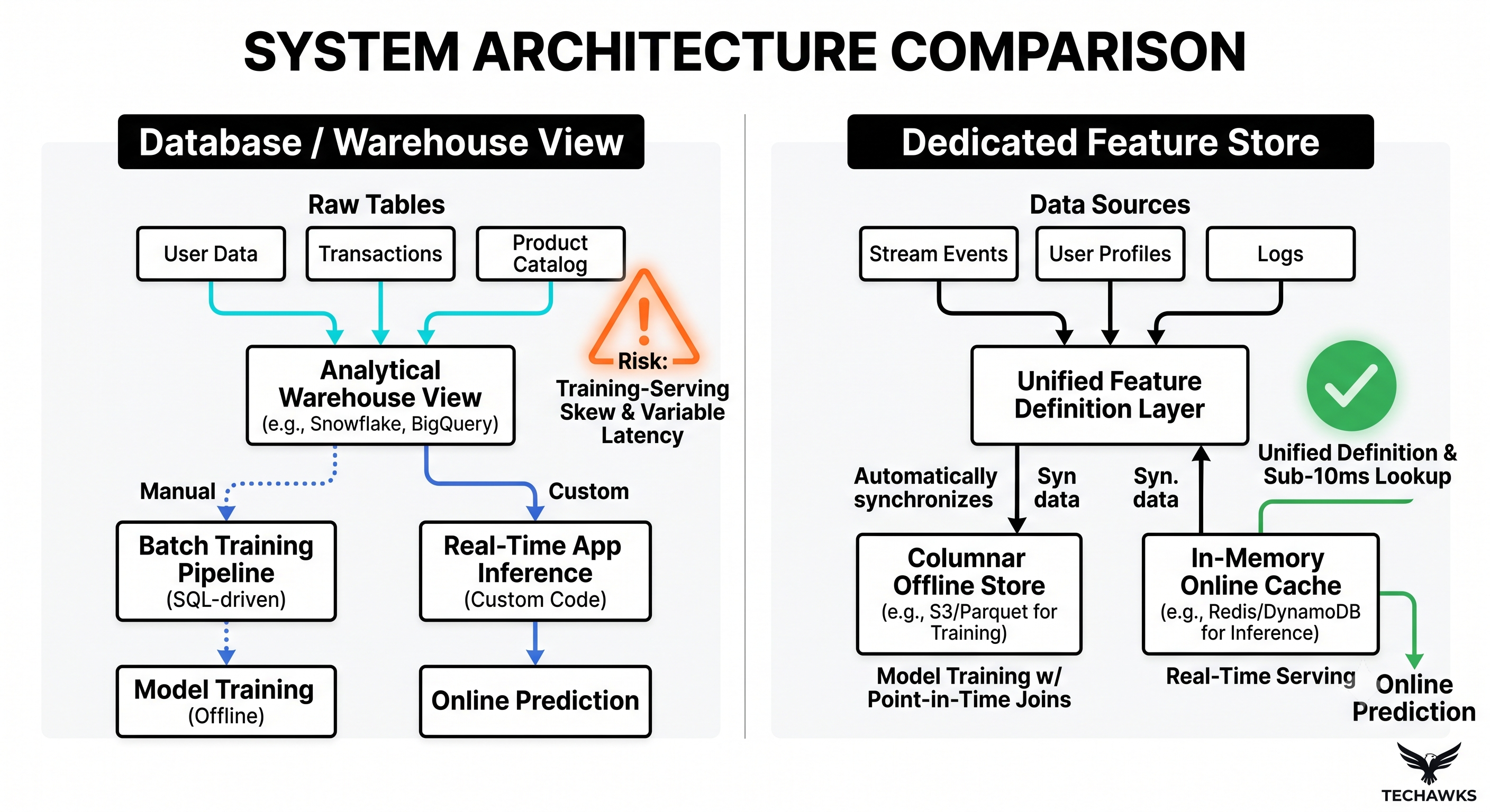 0 Commentaires 0 Parts 72 Vue 0 Aperçu
 -
The Vector-Only Trap: Why Enterprise Analytics Teams Are Rebuilding Lakehouses for Hybrid GraphRAG
For two years, data teams rushed to embed enterprise lakehouses into isolated vector databases. While pure cosine similarity handles fuzzy semantic lookup well, it fails on analytical reasoning.
If an analyst or autonomous agent asks: "Which enterprise accounts within two hops of our top churned customer experienced service degradation following last month's schema migration?"—vector similarity returns irrelevant documentation chunks. It cannot traverse foreign keys, entity relationships, or temporal causality.
To bridge the gap between unstructured knowledge and enterprise data lakes (Delta Lake, Apache Iceberg), modern data architectures are transitioning from naive vector retrieval to Hybrid GraphRAG (Knowledge Graph + Vector + Lakehouse):
1. The Dual Failure of Pure Vector vs. Pure SQL
Vector Alone: Treats enterprise data as isolated paragraphs, blinding models to topological relationships, parent-child hierarchies, and aggregate metrics.
SQL Alone: Rigid and brittle against messy natural language, unstructured notes, and semantic intent.
The Hybrid Solution: GraphRAG constructs an explicit semantic layer on top of your lakehouse. Entities (Accounts, Microservices, Incidents, Transactions) become nodes, and relational foreign keys or inferred interactions become edges, indexed alongside dense vector embeddings.
2. Asymmetric Dual-Channel Retrieval at Query Time
Instead of sending a single prompt to a vector index, production retrieval engines execute two concurrent passes:
The Local Vector Pass: Performs dense embedding retrieval to identify relevant unstructured text snippets and specific entry-point entity IDs.
The Global Graph Traversal: Runs Cypher/Gremlin sub-graph traversals (e.g., Personalized PageRank or community sub-clustering) starting from those entry-point nodes to collect multi-hop dependencies and historical lineage.
Context Fusion: Both streams are merged, deduplicated, and passed into a cross-encoder reranker before entering the LLM’s context window.
3. Direct Integration with Open Lakehouse Formats
The biggest architectural change is where this graph lives. Rather than maintaining brittle ETL pipelines syncing data into disconnected third-party vector and graph silos, data teams are querying graph views and embeddings directly over open table formats like Apache Iceberg. Graph engines now map directly to Parquet files via unified catalogs (such as Apache Polaris), enabling ACID guarantees, schema evolution, and time-travel rollbacks without data duplication.
Discussion Question
For data scientists, analytics engineers, and lakehouse architects: Has your team hit the limits of standard vector search in production? Are you actively layering Knowledge Graphs (GraphRAG) and hybrid search over your warehouse tables, or are relational SQL-to-text pipelines still handling your analytical queries?
CTA (Invite analysis and opinions)
Drop your thoughts, architecture diagrams, or benchmarks comparing vector vs. graph retrieval below. Let's analyze what real-world data pipelines look like at scale!The Vector-Only Trap: Why Enterprise Analytics Teams Are Rebuilding Lakehouses for Hybrid GraphRAG For two years, data teams rushed to embed enterprise lakehouses into isolated vector databases. While pure cosine similarity handles fuzzy semantic lookup well, it fails on analytical reasoning. If an analyst or autonomous agent asks: "Which enterprise accounts within two hops of our top churned customer experienced service degradation following last month's schema migration?"—vector similarity returns irrelevant documentation chunks. It cannot traverse foreign keys, entity relationships, or temporal causality. To bridge the gap between unstructured knowledge and enterprise data lakes (Delta Lake, Apache Iceberg), modern data architectures are transitioning from naive vector retrieval to Hybrid GraphRAG (Knowledge Graph + Vector + Lakehouse): 1. The Dual Failure of Pure Vector vs. Pure SQL Vector Alone: Treats enterprise data as isolated paragraphs, blinding models to topological relationships, parent-child hierarchies, and aggregate metrics. SQL Alone: Rigid and brittle against messy natural language, unstructured notes, and semantic intent. The Hybrid Solution: GraphRAG constructs an explicit semantic layer on top of your lakehouse. Entities (Accounts, Microservices, Incidents, Transactions) become nodes, and relational foreign keys or inferred interactions become edges, indexed alongside dense vector embeddings. 2. Asymmetric Dual-Channel Retrieval at Query Time Instead of sending a single prompt to a vector index, production retrieval engines execute two concurrent passes: The Local Vector Pass: Performs dense embedding retrieval to identify relevant unstructured text snippets and specific entry-point entity IDs. The Global Graph Traversal: Runs Cypher/Gremlin sub-graph traversals (e.g., Personalized PageRank or community sub-clustering) starting from those entry-point nodes to collect multi-hop dependencies and historical lineage. Context Fusion: Both streams are merged, deduplicated, and passed into a cross-encoder reranker before entering the LLM’s context window. 3. Direct Integration with Open Lakehouse Formats The biggest architectural change is where this graph lives. Rather than maintaining brittle ETL pipelines syncing data into disconnected third-party vector and graph silos, data teams are querying graph views and embeddings directly over open table formats like Apache Iceberg. Graph engines now map directly to Parquet files via unified catalogs (such as Apache Polaris), enabling ACID guarantees, schema evolution, and time-travel rollbacks without data duplication. Discussion Question For data scientists, analytics engineers, and lakehouse architects: Has your team hit the limits of standard vector search in production? Are you actively layering Knowledge Graphs (GraphRAG) and hybrid search over your warehouse tables, or are relational SQL-to-text pipelines still handling your analytical queries? CTA (Invite analysis and opinions) Drop your thoughts, architecture diagrams, or benchmarks comparing vector vs. graph retrieval below. Let's analyze what real-world data pipelines look like at scale! 0 Commentaires 0 Parts 16 Vue 0 Aperçu
 -
Detecting Silent Model Decay: A Production Guide to Quantifying Data & Concept Drift
In real-world data science, models rarely fail loudly with crash stack traces. They degrade silently because the statistical distribution of the incoming production features or the underlying relationship between inputs and targets shifts over time.
Relying on quarterly manual re-evaluations is too slow, and waiting for ground-truth labels can take weeks or months. Production data engineering requires an automated, statistical telemetry pipeline to catch drift in flight.
Here is a practical, step-by-step tutorial on implementing statistical drift detection for live inference pipelines.1. Separate Covariate Shift from Concept Shift Before choosing metrics, isolate the exact failure mode you are monitoring:
Covariate (Feature) Shift: The distribution of inputs changes ($P(X)$ changes), but the conditional relationship $P(Y \mid X)$ remains intact (e.g., user demographics skew younger, but purchasing behavior per age group remains stable).Concept Shift: The relationship between features and labels changes ($P(Y \mid X)$ changes), even if input distributions look identical (e.g., macroeconomic inflation changes what constitutes a "high-risk" loan amount).Prior Probability Shift: The target distribution changes ($P(Y)$ changes), common during seasonal demand spikes.2. Implement Statistical Distance Tests per Feature Type Never use simple mean and variance checks—they easily mask multimodal distributions and variance spikes. Segment your feature store into two testing tracks:
Continuous Features (Kolmogorov-Smirnov & Wasserstein Distance):Use the two-sample Kolmogorov-Smirnov (KS) test to compare the cumulative distribution function (CDF) of production samples against your training baseline.
Supplement with Wasserstein (Earth Mover's) Distance for an absolute, unit-interpretable metric indicating the work needed to transform the production distribution into the baseline.
Categorical Features (Population Stability Index - PSI):Group features into reference buckets and calculate PSI:$$\text{PSI} = \sum \left( \% \text{ Actual} - \% \text{ Expected} \right) \times \ln\left( \frac{\% \text{ Actual}}{\% \text{ Expected}} \right)$$Evaluation Rules:$\text{PSI} < 0.1$: Distribution stable; no action needed.$0.1 \le \text{PSI} < 0.25$: Moderate drift; flag for inspection.$\text{PSI} \ge 0.25$: Significant shift; trigger alert and review pipeline.3. Mitigate Sample Size Sensitivity with Windowed Baselines Statistical tests (like KS and Chi-square) are notoriously sensitive to huge sample sizes: with 500,000 requests, even a trivial, harmless fluctuation yields $p < 0.001$.Use sliding time windows (e.g., rolling 7-day batches) compared against a curated reference window (the model’s gold validation set) rather than an expanding historic pool.
Rely on effect-size metrics (such as PSI or normalized Wasserstein distance) as your primary alert triggers, using $p$-values strictly as secondary filters.4. Wire Drift Thresholds to Automated Retraining Triggers Drift detection is only valuable if it drives operational action:
When multiple critical features breach $\text{PSI} \ge 0.25$, trigger an automated pipeline (via Airflow, Prefect, or Kubeflow) to pull fresh labeled ground truth from recent partitions.
Automatically retrain a shadow candidate model, evaluate performance against current production data, and publish a comparative evaluation report before human sign-off on promotion.
Key Takeaways
Differentiate Shifts: Identify whether you are fighting feature distribution drift ($P(X)$) or fundamental concept decay ($P(Y \mid X)$).Pick the Right Test: Use KS/Wasserstein for continuous features and Population Stability Index (PSI) for categorical inputs.
Effect Size Over $p$-values: Avoid false alarms caused by sample size inflation by alerting on effect sizes ($\text{PSI} > 0.2\() rather than raw\)p$-values.
Automate the Feedback Loop: Connect statistical alerts directly to shadow retraining and validation pipelines.
CTA
How do you track silent model degradation in your production pipelines?Do you rely on dedicated open-source drift frameworks (like Evidently AI, Great Expectations, or NannyML), custom statistical scripts, or downstream business KPIs? Share your monitoring setup, threshold heuristics, and failure stories below.Detecting Silent Model Decay: A Production Guide to Quantifying Data & Concept Drift In real-world data science, models rarely fail loudly with crash stack traces. They degrade silently because the statistical distribution of the incoming production features or the underlying relationship between inputs and targets shifts over time. Relying on quarterly manual re-evaluations is too slow, and waiting for ground-truth labels can take weeks or months. Production data engineering requires an automated, statistical telemetry pipeline to catch drift in flight. Here is a practical, step-by-step tutorial on implementing statistical drift detection for live inference pipelines.1. Separate Covariate Shift from Concept Shift Before choosing metrics, isolate the exact failure mode you are monitoring: Covariate (Feature) Shift: The distribution of inputs changes ($P(X)$ changes), but the conditional relationship $P(Y \mid X)$ remains intact (e.g., user demographics skew younger, but purchasing behavior per age group remains stable).Concept Shift: The relationship between features and labels changes ($P(Y \mid X)$ changes), even if input distributions look identical (e.g., macroeconomic inflation changes what constitutes a "high-risk" loan amount).Prior Probability Shift: The target distribution changes ($P(Y)$ changes), common during seasonal demand spikes.2. Implement Statistical Distance Tests per Feature Type Never use simple mean and variance checks—they easily mask multimodal distributions and variance spikes. Segment your feature store into two testing tracks: Continuous Features (Kolmogorov-Smirnov & Wasserstein Distance):Use the two-sample Kolmogorov-Smirnov (KS) test to compare the cumulative distribution function (CDF) of production samples against your training baseline. Supplement with Wasserstein (Earth Mover's) Distance for an absolute, unit-interpretable metric indicating the work needed to transform the production distribution into the baseline. Categorical Features (Population Stability Index - PSI):Group features into reference buckets and calculate PSI:$$\text{PSI} = \sum \left( \% \text{ Actual} - \% \text{ Expected} \right) \times \ln\left( \frac{\% \text{ Actual}}{\% \text{ Expected}} \right)$$Evaluation Rules:$\text{PSI} < 0.1$: Distribution stable; no action needed.$0.1 \le \text{PSI} < 0.25$: Moderate drift; flag for inspection.$\text{PSI} \ge 0.25$: Significant shift; trigger alert and review pipeline.3. Mitigate Sample Size Sensitivity with Windowed Baselines Statistical tests (like KS and Chi-square) are notoriously sensitive to huge sample sizes: with 500,000 requests, even a trivial, harmless fluctuation yields $p < 0.001$.Use sliding time windows (e.g., rolling 7-day batches) compared against a curated reference window (the model’s gold validation set) rather than an expanding historic pool. Rely on effect-size metrics (such as PSI or normalized Wasserstein distance) as your primary alert triggers, using $p$-values strictly as secondary filters.4. Wire Drift Thresholds to Automated Retraining Triggers Drift detection is only valuable if it drives operational action: When multiple critical features breach $\text{PSI} \ge 0.25$, trigger an automated pipeline (via Airflow, Prefect, or Kubeflow) to pull fresh labeled ground truth from recent partitions. Automatically retrain a shadow candidate model, evaluate performance against current production data, and publish a comparative evaluation report before human sign-off on promotion. Key Takeaways Differentiate Shifts: Identify whether you are fighting feature distribution drift ($P(X)$) or fundamental concept decay ($P(Y \mid X)$).Pick the Right Test: Use KS/Wasserstein for continuous features and Population Stability Index (PSI) for categorical inputs. Effect Size Over $p$-values: Avoid false alarms caused by sample size inflation by alerting on effect sizes ($\text{PSI} > 0.2\() rather than raw\)p$-values. Automate the Feedback Loop: Connect statistical alerts directly to shadow retraining and validation pipelines. CTA How do you track silent model degradation in your production pipelines?Do you rely on dedicated open-source drift frameworks (like Evidently AI, Great Expectations, or NannyML), custom statistical scripts, or downstream business KPIs? Share your monitoring setup, threshold heuristics, and failure stories below.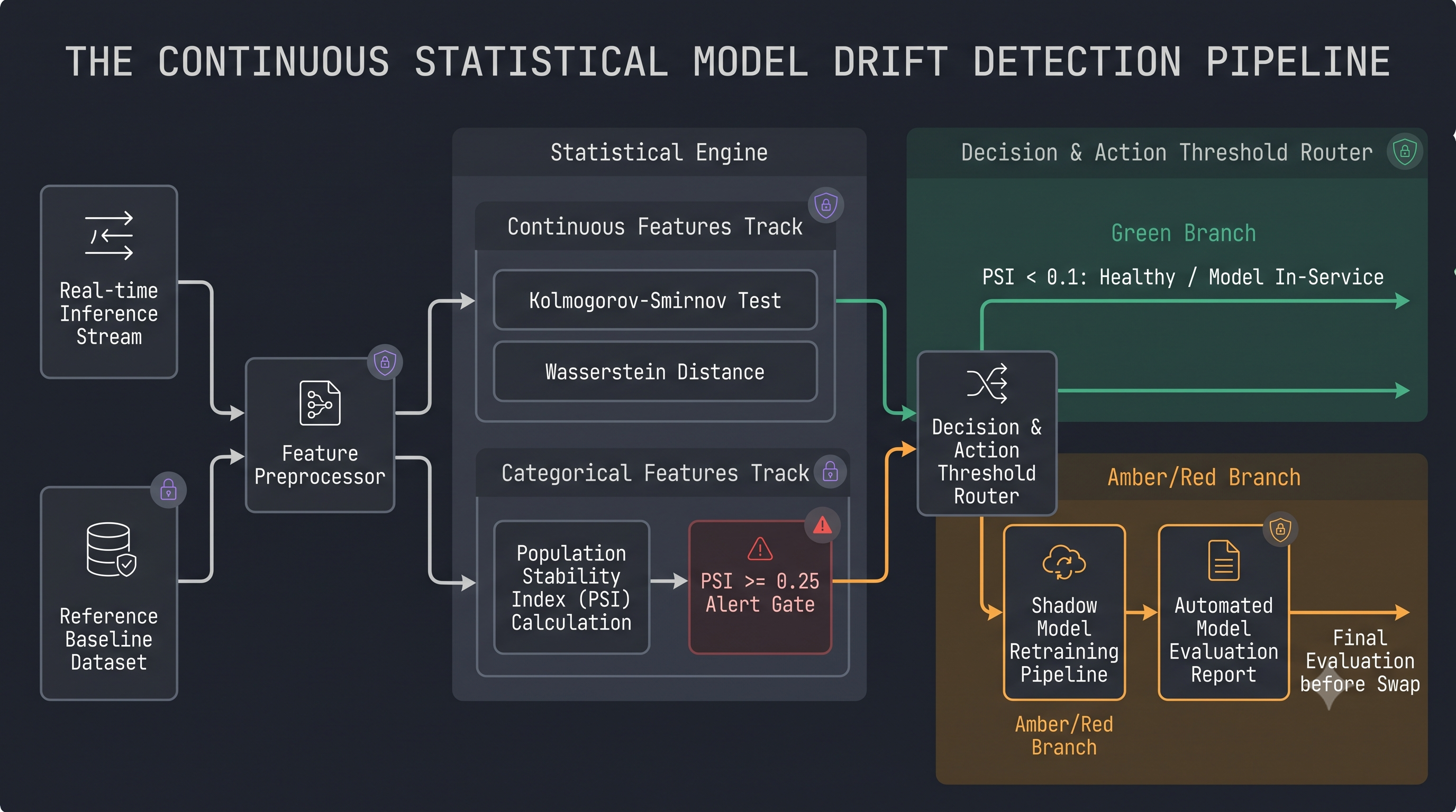 0 Commentaires 0 Parts 40 Vue 0 Aperçu
 -
The Silent Pipeline Killer: Why Isolated Drift Alerts Are Ruining Production ML (And How to Fix Your MLOps Stack)
Enterprise analytics and ML systems are managing unprecedented streaming throughput, with over 80% of organizations now deploying AI-augmented and real-time inference pipelines. Yet the biggest operational failure in production ML remains unchanged: treating statistical input drift ($P(X)$) as an automatic crisis without verifying concept drift or downstream evaluation impact ($P(Y\vert{}X)$).When a feature distribution shifts—such as a seasonal traffic spike skewing session lengths—a standard statistical test (KS test, Chi-square, or PSI > 0.2) triggers an alert. But if the relationship between input features and target predictions holds steady, triggering an emergency retrain wastes compute, disrupts feature stores, and risks model degradation on an under-sampled distribution.
Production-grade data teams in 2026 are shifting to eval-correlated drift monitoring. Instead of treating drift in isolation, run this verification checklist before retraining or rolling back models:📊 The Production Drift & Pipeline Triage Checklist
[ ] 1. Upstream Pipeline Audit vs. Real Shift: Before suspecting true behavioral drift, check upstream extraction. Did a schema alteration, timezone ingestion discrepancy, or upstream API null-filling bug artificially distort the feature distribution?
[ ] 2. Covariate vs. Concept Verification: Test whether $P(X)$ shifted while $P(Y\vert{}X)$ stayed stable (covariate shift), or if the underlying label boundary changed (concept drift). If only the input distribution shifted, sample reweighting or importance weighting is often faster, safer, and cheaper than a full retrain.
[ ] 3. Joint Eval-Trigger Validation: Configure alerting thresholds so on-call engineers are notified only when an input drift metric (e.g., PSI > 0.2 or Wasserstein distance) correlates directly with a measurable downstream evaluation drop (e.g., ground-truth conversion, precision dip, or LLM grounding degradation).
[ ] 4. Shadow & Canary Deployment Test: Never deploy an automated retrain directly to 100% of production traffic. Replay historical production traces against a canary model and compare performance across the drifted data slices specifically.[ ] 5. Feedback Loop & Stale Label Check: In delayed-feedback environments (like fraud detection or credit underwriting), verify whether apparent drift is simply unobserved ground-truth labels lagging behind inference windows.
Discussion Question
When your data pipelines or ML monitors detect a distribution shift, what criteria triggers an automatic model retraining job versus an engineer’s manual sign-off? How do you prevent statistical false alarms from burning out your team?
CTA (Invite Analysis and Opinions)
Drop your take below: Are you leaning toward automated closed-loop remediation, or do you still keep a human in the loop for pipeline intervention? If you have an active monitoring architecture, share your preferred drift detection metrics (PSI, KS test, or embedding distance).The Silent Pipeline Killer: Why Isolated Drift Alerts Are Ruining Production ML (And How to Fix Your MLOps Stack) Enterprise analytics and ML systems are managing unprecedented streaming throughput, with over 80% of organizations now deploying AI-augmented and real-time inference pipelines. Yet the biggest operational failure in production ML remains unchanged: treating statistical input drift ($P(X)$) as an automatic crisis without verifying concept drift or downstream evaluation impact ($P(Y\vert{}X)$).When a feature distribution shifts—such as a seasonal traffic spike skewing session lengths—a standard statistical test (KS test, Chi-square, or PSI > 0.2) triggers an alert. But if the relationship between input features and target predictions holds steady, triggering an emergency retrain wastes compute, disrupts feature stores, and risks model degradation on an under-sampled distribution. Production-grade data teams in 2026 are shifting to eval-correlated drift monitoring. Instead of treating drift in isolation, run this verification checklist before retraining or rolling back models:📊 The Production Drift & Pipeline Triage Checklist [ ] 1. Upstream Pipeline Audit vs. Real Shift: Before suspecting true behavioral drift, check upstream extraction. Did a schema alteration, timezone ingestion discrepancy, or upstream API null-filling bug artificially distort the feature distribution? [ ] 2. Covariate vs. Concept Verification: Test whether $P(X)$ shifted while $P(Y\vert{}X)$ stayed stable (covariate shift), or if the underlying label boundary changed (concept drift). If only the input distribution shifted, sample reweighting or importance weighting is often faster, safer, and cheaper than a full retrain. [ ] 3. Joint Eval-Trigger Validation: Configure alerting thresholds so on-call engineers are notified only when an input drift metric (e.g., PSI > 0.2 or Wasserstein distance) correlates directly with a measurable downstream evaluation drop (e.g., ground-truth conversion, precision dip, or LLM grounding degradation). [ ] 4. Shadow & Canary Deployment Test: Never deploy an automated retrain directly to 100% of production traffic. Replay historical production traces against a canary model and compare performance across the drifted data slices specifically.[ ] 5. Feedback Loop & Stale Label Check: In delayed-feedback environments (like fraud detection or credit underwriting), verify whether apparent drift is simply unobserved ground-truth labels lagging behind inference windows. Discussion Question When your data pipelines or ML monitors detect a distribution shift, what criteria triggers an automatic model retraining job versus an engineer’s manual sign-off? How do you prevent statistical false alarms from burning out your team? CTA (Invite Analysis and Opinions) Drop your take below: Are you leaning toward automated closed-loop remediation, or do you still keep a human in the loop for pipeline intervention? If you have an active monitoring architecture, share your preferred drift detection metrics (PSI, KS test, or embedding distance).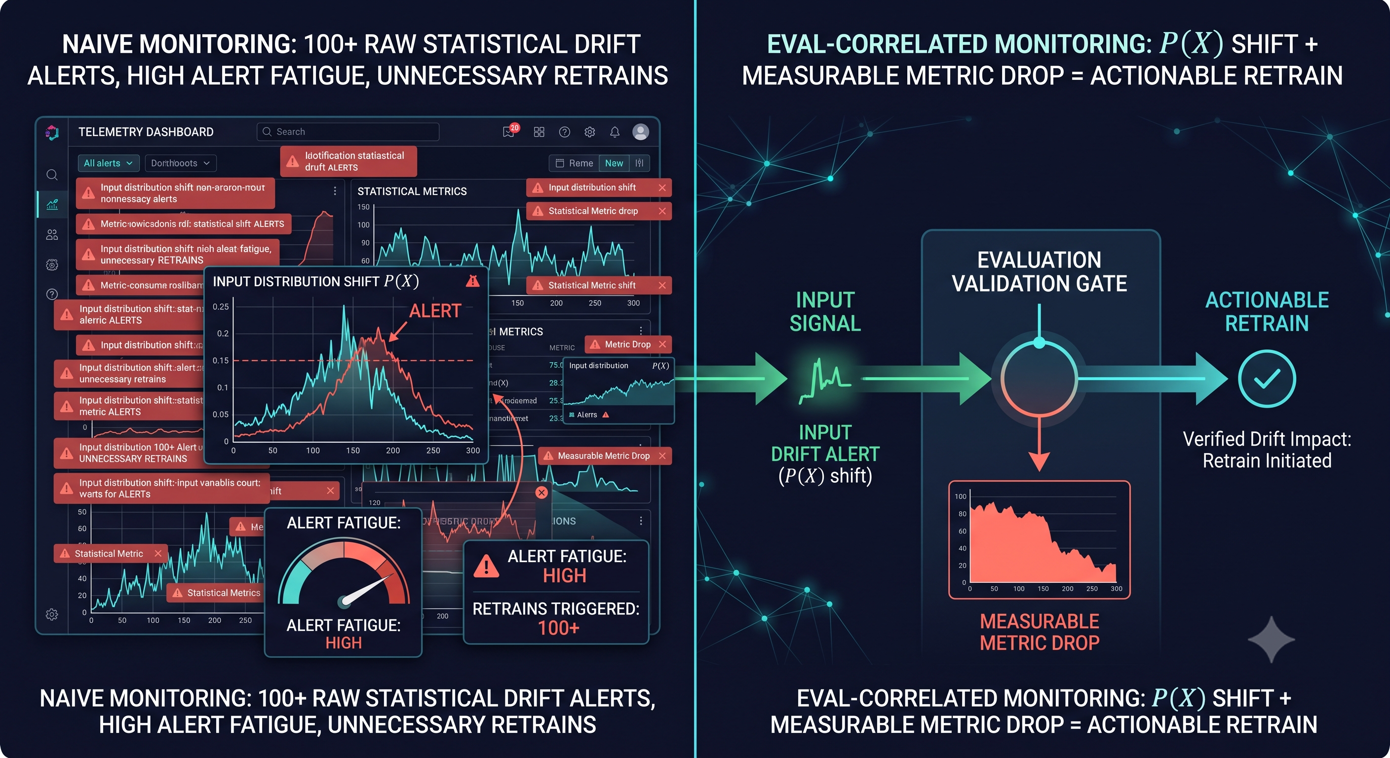 0 Commentaires 0 Parts 20 Vue 0 Aperçu
 -
Can Your Feature Store Detect Training-Serving Skew in Real Time? The 24-Hour Silent Drift Challenge.
In production ML systems, raw model architecture matters far less than data consistency across the serving boundary. When offline training batches use point-in-time joins that differ even slightly from real-time streaming feature transformations, training-serving skew corrupts your inference results while pipelines report 100% health.
Take the Techawks 24-Hour Data Pipeline Challenge to audit whether your data stack catches silent feature corruption before downstream systems ingest faulty predictions:
Audit Point-in-Time Correctness (Time-Travel Joins)
The Problem: Joining feature tables on static entity IDs without strict timestamp boundaries introduces subtle data leakage from future events into historical training sets, inflating offline accuracy metrics.
The Fix: Enforce point-in-time correct joins (AS-OF joins) in your feature store. Ensure every historical training observation only joins with feature values timestamped strictly prior to the observation event.
Benchmark Online vs. Offline Transformation Parity
The Problem: Re-implementing feature logic across different runtimes—such as running SQL/Spark for batch model training and rewriting the same logic in Python/Go for real-time API inference—creates discrepancies in null handling, string tokenization, or numerical scaling.
The Fix: Unify the transformation engine using a single declarative feature definition (via Feast, Hopsworks, or dbt/DuckDB engines) that compiles identical logic for both batch backfills and low-latency key-value stores (Redis/DynamoDB).
Deploy Statistical Drift Alarms on Streaming Ingress
The Problem: Traditional monitoring tracks system health metrics (latency, HTTP 500s, CPU usage) while ignoring distributional shifts in input features (e.g., changes in mean, variance, or categorical cardinality).
The Fix: Implement streaming Kolmogorov-Smirnov (K-S) or Population Stability Index (PSI) tests on real-time inference payloads. Set automated alerts to trip when input feature distributions deviate past a 0.1 PSI threshold compared to the baseline training distribution.
Key Takeaways
Time-Travel Hygiene Is Non-Negotiable: If your training pipeline doesn't enforce strict event-timestamp joins, your offline performance metrics are compromised by data leakage.
One Feature Definition, Two Storage Engines: Never maintain two separate codebases for offline batch features and online serving lookups.
Distributional Shift Is a Critical Bug: Monitor feature data drift with the same alerting rigor applied to API latency and 5xx errors.
CTA (Invite analysis and opinions)
How does your data team guard against training-serving skew and silent pipeline drift?
Do you enforce unified feature stores (like Feast or Hopsworks), or do you rely on custom microservice transformation layers?
What statistical drift thresholds or monitoring tools (e.g., Evidently AI, Great Expectations, Whylabs) have proven most dependable in your production stack?
Share your pipeline trade-offs and battle-tested strategies below!Can Your Feature Store Detect Training-Serving Skew in Real Time? The 24-Hour Silent Drift Challenge. In production ML systems, raw model architecture matters far less than data consistency across the serving boundary. When offline training batches use point-in-time joins that differ even slightly from real-time streaming feature transformations, training-serving skew corrupts your inference results while pipelines report 100% health. Take the Techawks 24-Hour Data Pipeline Challenge to audit whether your data stack catches silent feature corruption before downstream systems ingest faulty predictions: Audit Point-in-Time Correctness (Time-Travel Joins) The Problem: Joining feature tables on static entity IDs without strict timestamp boundaries introduces subtle data leakage from future events into historical training sets, inflating offline accuracy metrics. The Fix: Enforce point-in-time correct joins (AS-OF joins) in your feature store. Ensure every historical training observation only joins with feature values timestamped strictly prior to the observation event. Benchmark Online vs. Offline Transformation Parity The Problem: Re-implementing feature logic across different runtimes—such as running SQL/Spark for batch model training and rewriting the same logic in Python/Go for real-time API inference—creates discrepancies in null handling, string tokenization, or numerical scaling. The Fix: Unify the transformation engine using a single declarative feature definition (via Feast, Hopsworks, or dbt/DuckDB engines) that compiles identical logic for both batch backfills and low-latency key-value stores (Redis/DynamoDB). Deploy Statistical Drift Alarms on Streaming Ingress The Problem: Traditional monitoring tracks system health metrics (latency, HTTP 500s, CPU usage) while ignoring distributional shifts in input features (e.g., changes in mean, variance, or categorical cardinality). The Fix: Implement streaming Kolmogorov-Smirnov (K-S) or Population Stability Index (PSI) tests on real-time inference payloads. Set automated alerts to trip when input feature distributions deviate past a 0.1 PSI threshold compared to the baseline training distribution. Key Takeaways Time-Travel Hygiene Is Non-Negotiable: If your training pipeline doesn't enforce strict event-timestamp joins, your offline performance metrics are compromised by data leakage. One Feature Definition, Two Storage Engines: Never maintain two separate codebases for offline batch features and online serving lookups. Distributional Shift Is a Critical Bug: Monitor feature data drift with the same alerting rigor applied to API latency and 5xx errors. CTA (Invite analysis and opinions) How does your data team guard against training-serving skew and silent pipeline drift? Do you enforce unified feature stores (like Feast or Hopsworks), or do you rely on custom microservice transformation layers? What statistical drift thresholds or monitoring tools (e.g., Evidently AI, Great Expectations, Whylabs) have proven most dependable in your production stack? Share your pipeline trade-offs and battle-tested strategies below!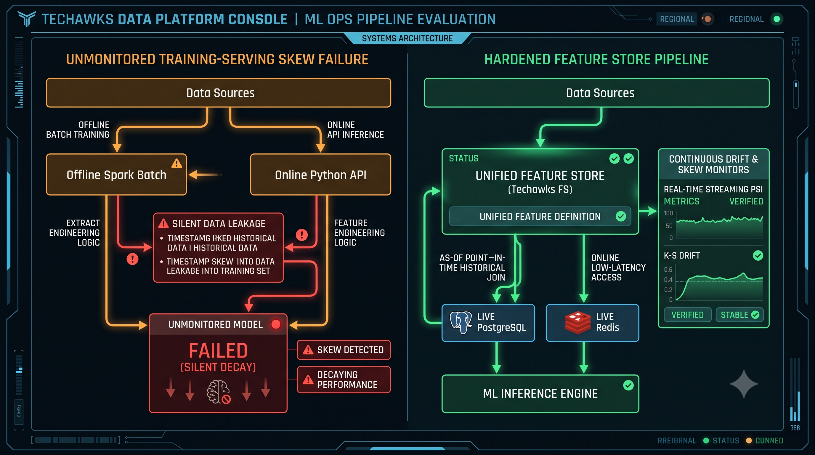 0 Commentaires 0 Parts 68 Vue 0 Aperçu
 -
Myth vs Fact: Can Synthetic Data Completely Replace Real Production Data?
Synthetic data is an invaluable amplifier, but confusing simulated distributions with ground-truth production behavior breaks real systems:
❌ Myth 1: "Synthetic data solves data quality because it eliminates real-world noise.
"The Reality: Real-world noise is often where the signal lives. Real datasets contain edge-case anomalies, sensor dropouts, regional formatting nuances, and subtle user behavior shifts. When you generate synthetic data using a parametric model or an LLM, the synthesizer only samples from its own internal representations. In eliminating "noise," you often scrub out the exact low-frequency, high-impact tail events (such as novel fraud vectors or rare hardware failures) that determine whether a production model survives in the wild.
❌ Myth 2: "Training models recursively on synthetic data creates an infinite data fly-wheel.
"The Reality: Recursive synthetic training leads directly to Model Collapse and variance loss. When generative models train on data generated by earlier generative models, the probability distribution's tails get trimmed with each successive generation. Over iterations, the model forgets rare categorical values, amplifies systemic biases, and collapses into modal collapse—producing uniform, uninformative outputs that degrade test-set generalization.
❌ Myth 3: "Synthetic data automatically guarantees complete privacy and regulatory compliance.
"The Reality: Generating synthetic rows does not grant an automatic privacy shield. Without formal Differential Privacy ($\epsilon, \delta$) guarantees, generative models (especially GANs, Diffusion models, and LLMs) can memorize outlier training examples. An adversarial membership inference attack or shadow-model reconstruction can extract verbatim confidential records from poorly regularized synthetic sets.
Where Synthetic Data Actually Belongs in Your Pipeline Cold-Start & Class Imbalance: Augmenting sparse minority classes (e.g., boosting a 0.01% rare medical anomaly or credit chargeback class to 2% for gradient stability).Stress-Testing & Adversarial Probing: Generating synthetic perturbations to evaluate model robustness and bias before deployment.
Privacy-Preserving Staging Environments: Creating high-fidelity, schema-valid mock databases so developers and external partners can build pipelines without touching raw production PII.
Discussion Question
For the data scientists, ML engineers, and analysts in our community: Where does synthetic data sit in your current stack? Are you actively using it for class balancing and CI/CD validation, or have you noticed synthetic data degrading model accuracy when deployed on live customer streams?
CTA
We want your analysis! Drop your methodology, benchmarks, or thoughts on managing model collapse vs. real-world data drift in the comments below. Let’s compare notes! 🦅📊Myth vs Fact: Can Synthetic Data Completely Replace Real Production Data? Synthetic data is an invaluable amplifier, but confusing simulated distributions with ground-truth production behavior breaks real systems: ❌ Myth 1: "Synthetic data solves data quality because it eliminates real-world noise. "The Reality: Real-world noise is often where the signal lives. Real datasets contain edge-case anomalies, sensor dropouts, regional formatting nuances, and subtle user behavior shifts. When you generate synthetic data using a parametric model or an LLM, the synthesizer only samples from its own internal representations. In eliminating "noise," you often scrub out the exact low-frequency, high-impact tail events (such as novel fraud vectors or rare hardware failures) that determine whether a production model survives in the wild. ❌ Myth 2: "Training models recursively on synthetic data creates an infinite data fly-wheel. "The Reality: Recursive synthetic training leads directly to Model Collapse and variance loss. When generative models train on data generated by earlier generative models, the probability distribution's tails get trimmed with each successive generation. Over iterations, the model forgets rare categorical values, amplifies systemic biases, and collapses into modal collapse—producing uniform, uninformative outputs that degrade test-set generalization. ❌ Myth 3: "Synthetic data automatically guarantees complete privacy and regulatory compliance. "The Reality: Generating synthetic rows does not grant an automatic privacy shield. Without formal Differential Privacy ($\epsilon, \delta$) guarantees, generative models (especially GANs, Diffusion models, and LLMs) can memorize outlier training examples. An adversarial membership inference attack or shadow-model reconstruction can extract verbatim confidential records from poorly regularized synthetic sets. Where Synthetic Data Actually Belongs in Your Pipeline Cold-Start & Class Imbalance: Augmenting sparse minority classes (e.g., boosting a 0.01% rare medical anomaly or credit chargeback class to 2% for gradient stability).Stress-Testing & Adversarial Probing: Generating synthetic perturbations to evaluate model robustness and bias before deployment. Privacy-Preserving Staging Environments: Creating high-fidelity, schema-valid mock databases so developers and external partners can build pipelines without touching raw production PII. Discussion Question For the data scientists, ML engineers, and analysts in our community: Where does synthetic data sit in your current stack? Are you actively using it for class balancing and CI/CD validation, or have you noticed synthetic data degrading model accuracy when deployed on live customer streams? CTA We want your analysis! Drop your methodology, benchmarks, or thoughts on managing model collapse vs. real-world data drift in the comments below. Let’s compare notes! 🦅📊 0 Commentaires 0 Parts 61 Vue 0 Aperçu
 -
Tool Review: Polars vs. Pandas—Is It Finally Time to Retire the Default DataFrame?
Pandas remains the lingua franca of tabular data manipulation, yet its single-threaded, eager execution model often requires painful workarounds like chunking or premature migration to distributed engines like Spark. Polars takes a radically different architectural approach: written in Rust, built on Apache Arrow, and powered by a lazy evaluation query optimizer with native multithreading.
Where Polars Wins:
Memory Efficiency & Zero-Copy: Because it leverages Arrow memory layouts, Polars handles contiguous memory efficiently and avoids unnecessary object duplication.
Lazy Execution Engine: With pl.scan_parquet() or pl.scan_csv(), Polars optimizes queries before touching data—pushing down predicates and selecting only required columns.
Predictable Syntax: By eliminating multi-indexes and index-based slicing, Polars enforces explicit, expression-based transformations that prevent silent slicing bugs.
Where Pandas Still Holds Ground:
Ecosystem Maturity: The vast majority of legacy ML libraries, specialized stats packages, and visualization tools expect Pandas or standard NumPy arrays natively.
Community Resources: Finding niche debugging solutions, custom extensions, and Stack Overflow answers is still effortless in Pandas compared to newer Polars patterns.
Learning Curve for SQL-Like Thinking: Polars discourages procedural row-by-row iteration in favor of columnar expressions, which requires unlearning years of df.apply() habits.
Key Takeaways
Scale locally first: Polars bridges the gap between single-machine analysis and expensive distributed clusters by maximizing multi-core CPU and memory usage.
Expressions over indices: Dropping explicit index tracking removes a major source of syntax confusion and performance bottlenecks.
Hybrid coexistence: You don't need an immediate full migration; converting from Polars to Pandas via PyArrow at the model boundary is nearly zero-cost.
CTA (Invite analysis and opinions)
If your team handles 5GB–50GB datasets on a single node: Have you made the shift to Polars in production pipelines, or is Pandas (especially with the PyArrow engine backend) still your default? What friction did your team face during the transition? Let’s hear your benchmarks and real-world trade-offs below.Tool Review: Polars vs. Pandas—Is It Finally Time to Retire the Default DataFrame? Pandas remains the lingua franca of tabular data manipulation, yet its single-threaded, eager execution model often requires painful workarounds like chunking or premature migration to distributed engines like Spark. Polars takes a radically different architectural approach: written in Rust, built on Apache Arrow, and powered by a lazy evaluation query optimizer with native multithreading. Where Polars Wins: Memory Efficiency & Zero-Copy: Because it leverages Arrow memory layouts, Polars handles contiguous memory efficiently and avoids unnecessary object duplication. Lazy Execution Engine: With pl.scan_parquet() or pl.scan_csv(), Polars optimizes queries before touching data—pushing down predicates and selecting only required columns. Predictable Syntax: By eliminating multi-indexes and index-based slicing, Polars enforces explicit, expression-based transformations that prevent silent slicing bugs. Where Pandas Still Holds Ground: Ecosystem Maturity: The vast majority of legacy ML libraries, specialized stats packages, and visualization tools expect Pandas or standard NumPy arrays natively. Community Resources: Finding niche debugging solutions, custom extensions, and Stack Overflow answers is still effortless in Pandas compared to newer Polars patterns. Learning Curve for SQL-Like Thinking: Polars discourages procedural row-by-row iteration in favor of columnar expressions, which requires unlearning years of df.apply() habits. Key Takeaways Scale locally first: Polars bridges the gap between single-machine analysis and expensive distributed clusters by maximizing multi-core CPU and memory usage. Expressions over indices: Dropping explicit index tracking removes a major source of syntax confusion and performance bottlenecks. Hybrid coexistence: You don't need an immediate full migration; converting from Polars to Pandas via PyArrow at the model boundary is nearly zero-cost. CTA (Invite analysis and opinions) If your team handles 5GB–50GB datasets on a single node: Have you made the shift to Polars in production pipelines, or is Pandas (especially with the PyArrow engine backend) still your default? What friction did your team face during the transition? Let’s hear your benchmarks and real-world trade-offs below.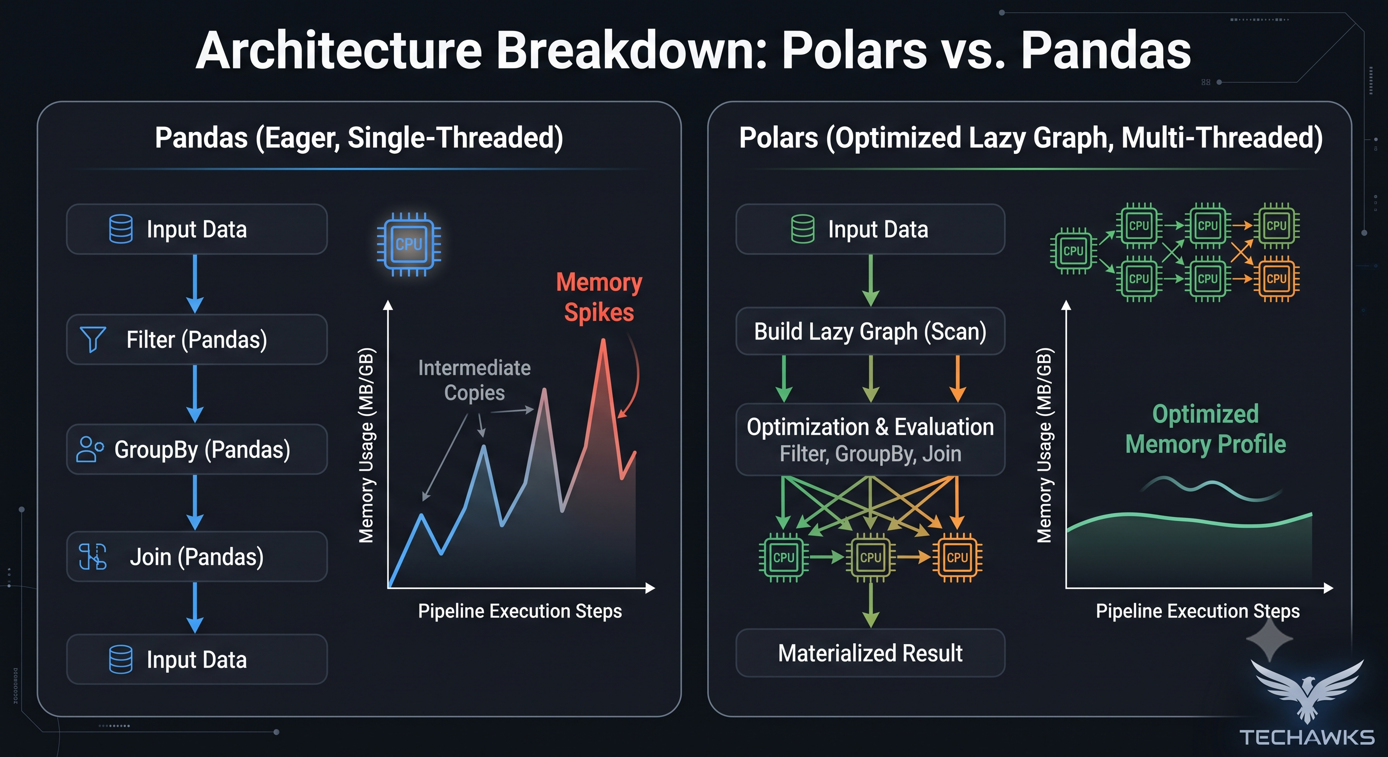 0 Commentaires 0 Parts 79 Vue 0 Aperçu
 -
Stop Writing SQL from Scratch: Why AI Agents Are Shifting the Value of Data Analysts in 2026
Over the past year, we have moved from generative AI as a "clever chatbot" to autonomous AI data agents directly integrated into the modern data stack.
Tools running across warehouses like Snowflake and BigQuery can now parse plain-English business requests, auto-generate complex multi-table joins, perform anomaly checks, and draft presentation slides in seconds.
Why This Matters to Your Career
Many data practitioners fear automation. But the real shift isn't job elimination; it is an aggressive change in where leverage lives:
Before: High value was placed on execution mechanics (writing syntax, tuning ETL queries, manually building boilerplate charts).
Now: Value has shifted entirely to semantic architecture, verification, and problem framing.
When an AI agent spits out a 45-line SQL query with a 15% revenue deviation anomaly, leadership does not need someone who can type faster. They need someone who understands whether the metric logic aligns with actual business operations, whether underlying data leakage skewed the inference, and what decision the CEO should make with that number.
The 3 Skills That Protect Your Value
Semantic Modeling & Data Contracts: Instead of building ad-hoc queries, high-earning analysts design the governed semantic layer (metrics definitions, standardized schemas) that AI agents rely on to avoid hallucinating business facts.
Contextual Auditing & Truth-Checking: AI writes syntactically valid code that is frequently contextually wrong. Knowing how to stress-test an agent's assumptions is the new code review.
Translational Storytelling: Connecting raw statistical output to capital allocation, cost reduction, or product roadmaps. Algorithms calculate; humans contextualize trade-offs.
Discussion Question
For those currently working in analytics and data science:
How much of your day-to-day query writing and dashboard maintenance has been handed off to AI tools, and what new high-leverage skill are you actively prioritizing this quarter?
CTA
Drop your workflow breakdown in the comments—are you seeing your company demand deeper domain reasoning and semantic modeling, or is traditional syntax-first reporting still the norm in your team? Let's analyze where the industry is truly heading versus the hype.Stop Writing SQL from Scratch: Why AI Agents Are Shifting the Value of Data Analysts in 2026 Over the past year, we have moved from generative AI as a "clever chatbot" to autonomous AI data agents directly integrated into the modern data stack. Tools running across warehouses like Snowflake and BigQuery can now parse plain-English business requests, auto-generate complex multi-table joins, perform anomaly checks, and draft presentation slides in seconds. Why This Matters to Your Career Many data practitioners fear automation. But the real shift isn't job elimination; it is an aggressive change in where leverage lives: Before: High value was placed on execution mechanics (writing syntax, tuning ETL queries, manually building boilerplate charts). Now: Value has shifted entirely to semantic architecture, verification, and problem framing. When an AI agent spits out a 45-line SQL query with a 15% revenue deviation anomaly, leadership does not need someone who can type faster. They need someone who understands whether the metric logic aligns with actual business operations, whether underlying data leakage skewed the inference, and what decision the CEO should make with that number. The 3 Skills That Protect Your Value Semantic Modeling & Data Contracts: Instead of building ad-hoc queries, high-earning analysts design the governed semantic layer (metrics definitions, standardized schemas) that AI agents rely on to avoid hallucinating business facts. Contextual Auditing & Truth-Checking: AI writes syntactically valid code that is frequently contextually wrong. Knowing how to stress-test an agent's assumptions is the new code review. Translational Storytelling: Connecting raw statistical output to capital allocation, cost reduction, or product roadmaps. Algorithms calculate; humans contextualize trade-offs. Discussion Question For those currently working in analytics and data science: How much of your day-to-day query writing and dashboard maintenance has been handed off to AI tools, and what new high-leverage skill are you actively prioritizing this quarter? CTA Drop your workflow breakdown in the comments—are you seeing your company demand deeper domain reasoning and semantic modeling, or is traditional syntax-first reporting still the norm in your team? Let's analyze where the industry is truly heading versus the hype. 0 Commentaires 0 Parts 71 Vue 0 Aperçu
 -
Where do most real-world data science projects actually stall out?
Building a high-performing model in a notebook is rarely the hardest part of delivering business value. The friction almost always emerges when bridging raw, messy source data to a reliable, monitored production environment.
Cast your vote below on the single biggest bottleneck you encounter in your data pipeline lifecycle:
A) Fragmented data quality & schema drift (upstream changes breaking pipelines silently)
B) Ambiguous business metrics (stakeholders cannot define a measurable objective function)
C) Feature store & deployment drift (training/serving skew and operational MLOps debt)
D) Organizational buy-in & adoption (a 95% accurate model that nobody trusts or integrates)
Select your vote above, then head to the comments. If you could eliminate just one of these hurdles from your daily workflow, which would yield the highest ROI for your team?
Key Takeaways
Data pipelines outweigh modeling: Robust data validation frameworks often generate higher business impact than incremental model accuracy gains.
Alignment prevents rework: A model optimized for the wrong KPI is dead on arrival, no matter how complex the architecture.
Serving requires dedicated observability: Monitoring for concept drift and distribution shifts is essential to keep production systems reliable over time.
CTA
Let’s hear your analysis: How is your team currently tackling silent pipeline failures and schema drift? Drop your battle-tested tools, automated validation strategies, or hardest lessons learned below.Where do most real-world data science projects actually stall out? Building a high-performing model in a notebook is rarely the hardest part of delivering business value. The friction almost always emerges when bridging raw, messy source data to a reliable, monitored production environment. Cast your vote below on the single biggest bottleneck you encounter in your data pipeline lifecycle: A) Fragmented data quality & schema drift (upstream changes breaking pipelines silently) B) Ambiguous business metrics (stakeholders cannot define a measurable objective function) C) Feature store & deployment drift (training/serving skew and operational MLOps debt) D) Organizational buy-in & adoption (a 95% accurate model that nobody trusts or integrates) Select your vote above, then head to the comments. If you could eliminate just one of these hurdles from your daily workflow, which would yield the highest ROI for your team? Key Takeaways Data pipelines outweigh modeling: Robust data validation frameworks often generate higher business impact than incremental model accuracy gains. Alignment prevents rework: A model optimized for the wrong KPI is dead on arrival, no matter how complex the architecture. Serving requires dedicated observability: Monitoring for concept drift and distribution shifts is essential to keep production systems reliable over time. CTA Let’s hear your analysis: How is your team currently tackling silent pipeline failures and schema drift? Drop your battle-tested tools, automated validation strategies, or hardest lessons learned below.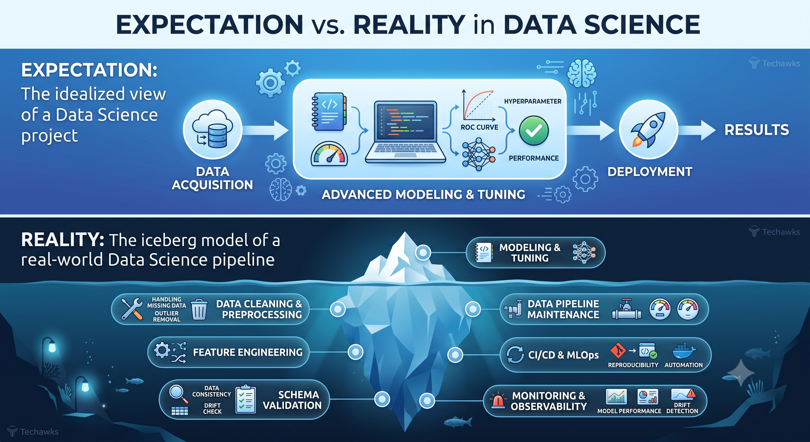 0 Commentaires 0 Parts 235 Vue 0 Aperçu
 -
The Golden Dataset Fallacy: Why Static Evaluation Is Silently Breaking Production AI
As engineering teams transition from classical tabular models to production RAG pipelines and conversational analytics agents, an uncomfortable truth has emerged across modern data platforms: static evaluation benchmarks actively lie over time.
Most data and ML teams test pipelines against a "golden dataset" established at launch. In classical predictive modeling, covariate shift is easily identified with statistical metrics like Population Stability Index (PSI) or Kolmogorov-Smirnov (KS) tests. However, in generative analytics and semantic query systems, data drift is multifaceted and insidious:
Retrieval-Corpus Drift: The production vector database updates continuously as enterprise data changes, but the benchmark queries still test against the baseline assumptions of day one.
Input Persona & Intent Drift: Real-world users phrase queries, edge cases, and analytical constraints entirely differently from the synthetic or curated test sets generated during development.
Prompt & Schema Mutation: Upstream database schema changes or subtle prompt adjustments subtly alter how SQL queries or answers are generated, bypassing baseline unit checks without triggering formal assertion errors.
When your CI/CD pipeline runs against an unversioned, frozen evaluation set, the score stays artificially flat while production utility rapidly decays.
Practical Resource: A 4-Step Eval-Drift Auditing Workflow
Stratified Trace Sampling: Sample 200–500 production queries across rolling 14-to-28-day windows. Cluster queries using semantic embeddings (e.g., HDBSCAN over prompt embeddings) to uncover unmapped customer intents that never existed in the original test suite.
Track Corpus-Query Desync: Ensure golden test cases explicitly log the vector corpus hash and chunk IDs retrieved during the test. If high-performing queries start fetching entirely different chunks in production, flag them for retrieval recalibration.
Continuous LLM-as-a-Judge Rubrics: Run automated evaluation runs scored on specific unit axes—Context Precision, Faithfulness/Groundedness, and Semantic Answer Relevance—rather than simple string matching or token similarity (ROUGE/BLEU).
Semantic Version Your Benchmarks: Treat test sets like production code (eval_golden_v2.4_2026_09). When a score drops after a dataset update, measure the variance to distinguish between true model regression and alignment with evolving real-world traffic.
Discussion Question
How frequently does your team refresh and re-baseline your evaluation datasets, and how do you separate true model degradation from underlying test-corpus drift?
CTA (Invite analysis and opinions)
Share your evaluation pipelines and drift-monitoring setups below. Let’s break down the best metrics for keeping validation suites honest against real-world production drift.The Golden Dataset Fallacy: Why Static Evaluation Is Silently Breaking Production AI As engineering teams transition from classical tabular models to production RAG pipelines and conversational analytics agents, an uncomfortable truth has emerged across modern data platforms: static evaluation benchmarks actively lie over time. Most data and ML teams test pipelines against a "golden dataset" established at launch. In classical predictive modeling, covariate shift is easily identified with statistical metrics like Population Stability Index (PSI) or Kolmogorov-Smirnov (KS) tests. However, in generative analytics and semantic query systems, data drift is multifaceted and insidious: Retrieval-Corpus Drift: The production vector database updates continuously as enterprise data changes, but the benchmark queries still test against the baseline assumptions of day one. Input Persona & Intent Drift: Real-world users phrase queries, edge cases, and analytical constraints entirely differently from the synthetic or curated test sets generated during development. Prompt & Schema Mutation: Upstream database schema changes or subtle prompt adjustments subtly alter how SQL queries or answers are generated, bypassing baseline unit checks without triggering formal assertion errors. When your CI/CD pipeline runs against an unversioned, frozen evaluation set, the score stays artificially flat while production utility rapidly decays. Practical Resource: A 4-Step Eval-Drift Auditing Workflow Stratified Trace Sampling: Sample 200–500 production queries across rolling 14-to-28-day windows. Cluster queries using semantic embeddings (e.g., HDBSCAN over prompt embeddings) to uncover unmapped customer intents that never existed in the original test suite. Track Corpus-Query Desync: Ensure golden test cases explicitly log the vector corpus hash and chunk IDs retrieved during the test. If high-performing queries start fetching entirely different chunks in production, flag them for retrieval recalibration. Continuous LLM-as-a-Judge Rubrics: Run automated evaluation runs scored on specific unit axes—Context Precision, Faithfulness/Groundedness, and Semantic Answer Relevance—rather than simple string matching or token similarity (ROUGE/BLEU). Semantic Version Your Benchmarks: Treat test sets like production code (eval_golden_v2.4_2026_09). When a score drops after a dataset update, measure the variance to distinguish between true model regression and alignment with evolving real-world traffic. Discussion Question How frequently does your team refresh and re-baseline your evaluation datasets, and how do you separate true model degradation from underlying test-corpus drift? CTA (Invite analysis and opinions) Share your evaluation pipelines and drift-monitoring setups below. Let’s break down the best metrics for keeping validation suites honest against real-world production drift.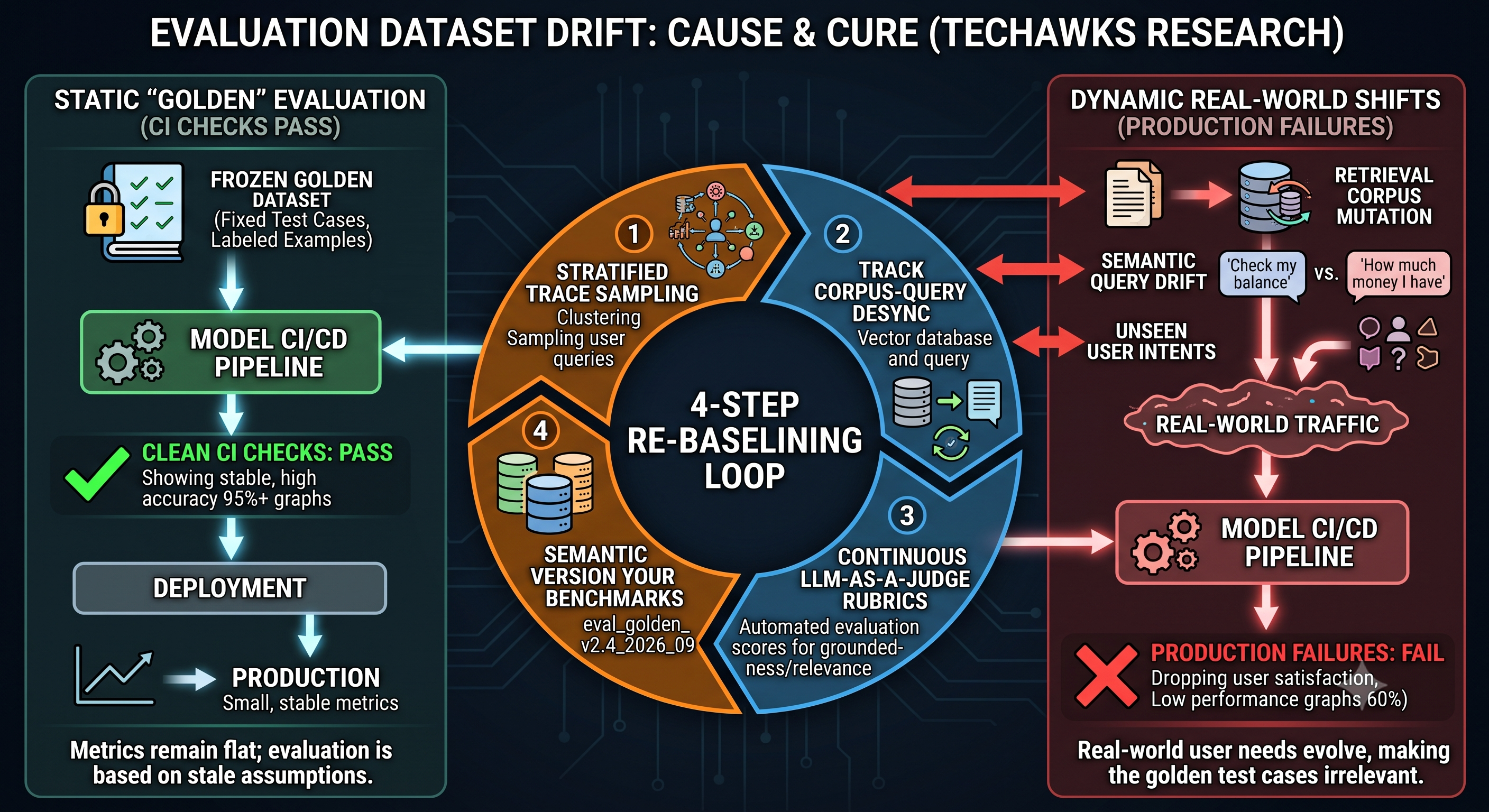 0 Commentaires 0 Parts 93 Vue 0 Aperçu
 -
The Accuracy Mirage: Why 98% Test Performance Fails in Production
Kaggle leaderboards and university courses train practitioners to maximize offline metrics like $R^2$, ROC-AUC, or F1 scores. In production, however, a mathematically elegant model is only as good as the reliability of its incoming data pipeline.
When analytical systems fail to deliver business value, the culprit is rarely model architecture:
Training-Serving Skew: Features computed offline over historical batches frequently diverge from real-time features generated during inference. If your feature transformations differ between development and runtime environments, your metrics mean nothing.
Silent Concept and Data Drift: Consumer behavior shifts, external markets fluctuate, and upstream schemas change without notification. Without automated drift detection and data validation checks (like Great Expectations or schema assertions), models fail silently while continuing to output confident predictions.
Optimizing for Metrics Instead of Value: A 1% increase in precision matters very little if latency increases tenfold or if the business team cannot interpret the decision boundary. Aligning the cost function directly with business KPIs—such as false positive remediation cost—trumps raw statistical elegance.
Real-world machine learning is roughly 10% modeling and 90% data engineering, monitoring, and pipeline hygiene.
Key Takeaways
Offline Metrics Don't Guarantee Live Success: High benchmark validation scores often mask data leakage or distribution shifts.
Invest in Monitoring Over Fine-Tuning: Continuous tracking of feature distribution and concept drift is critical for model longevity.
Bridge the Business Gap: Optimize for operational impact and explainability over incremental statistical gains.
CTA
Let’s hear your perspective and analysis:
What was the most painful or surprising way a model failed after being pushed to production in your experience?
What are your go-to practices or tools for catching data drift and maintaining data quality before inference breaks? Share your stack and opinions below.The Accuracy Mirage: Why 98% Test Performance Fails in Production Kaggle leaderboards and university courses train practitioners to maximize offline metrics like $R^2$, ROC-AUC, or F1 scores. In production, however, a mathematically elegant model is only as good as the reliability of its incoming data pipeline. When analytical systems fail to deliver business value, the culprit is rarely model architecture: Training-Serving Skew: Features computed offline over historical batches frequently diverge from real-time features generated during inference. If your feature transformations differ between development and runtime environments, your metrics mean nothing. Silent Concept and Data Drift: Consumer behavior shifts, external markets fluctuate, and upstream schemas change without notification. Without automated drift detection and data validation checks (like Great Expectations or schema assertions), models fail silently while continuing to output confident predictions. Optimizing for Metrics Instead of Value: A 1% increase in precision matters very little if latency increases tenfold or if the business team cannot interpret the decision boundary. Aligning the cost function directly with business KPIs—such as false positive remediation cost—trumps raw statistical elegance. Real-world machine learning is roughly 10% modeling and 90% data engineering, monitoring, and pipeline hygiene. Key Takeaways Offline Metrics Don't Guarantee Live Success: High benchmark validation scores often mask data leakage or distribution shifts. Invest in Monitoring Over Fine-Tuning: Continuous tracking of feature distribution and concept drift is critical for model longevity. Bridge the Business Gap: Optimize for operational impact and explainability over incremental statistical gains. CTA Let’s hear your perspective and analysis: What was the most painful or surprising way a model failed after being pushed to production in your experience? What are your go-to practices or tools for catching data drift and maintaining data quality before inference breaks? Share your stack and opinions below.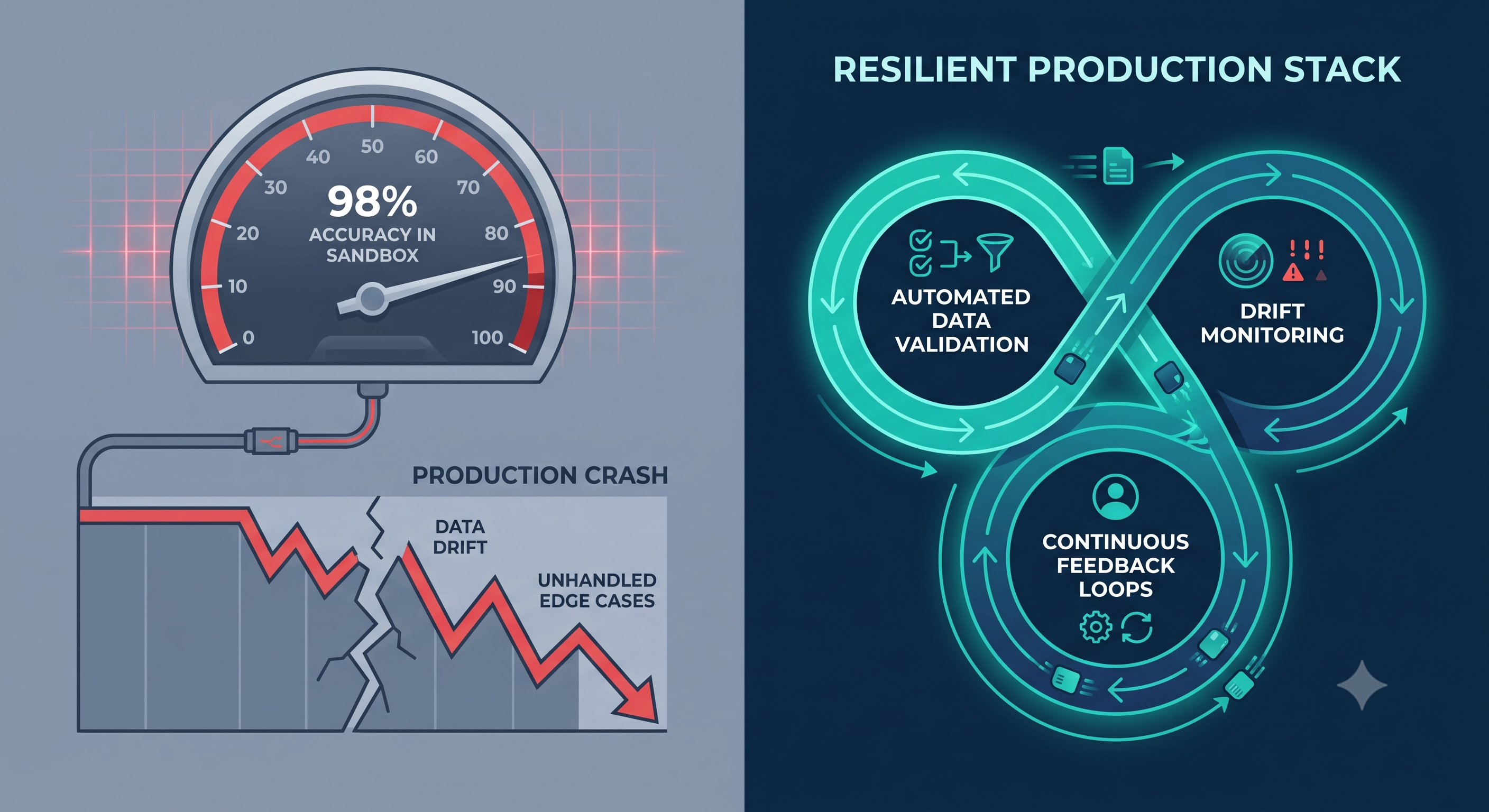 0 Commentaires 0 Parts 128 Vue 0 Aperçu
Plus de lecture